A Precise Vocabulary for System Understanding

The word context is overloaded in observability discourse to the point of losing precision. It is used to refer to shared labels, a topology map, temporal proximity, and propagated trace identifiers. Four distinct things, each useful, none of them sufficient.

This blog defines a precise, layered model of observability semantics intended for engineers and SREs building or operating complex distributed systems.

The Gap in Current Observability Tooling

Most observability tooling today implements a shallow semantics of entity and some form of topology, often referred to as the knowledge graph – typically derived from trace data – with partial reach into behavior through threshold-based alerting and anomaly detection. A knowledge graph is a generic term that does not define the semantics of what it captures. It is typically assumed to be a list of services and their topological relationships, but as we point out later, this is not sufficient to answer questions. It is also a dynamic, ever-changing graph; capturing it only once, or once a week, is not a reliable representation for real-time, continuous, automated operation. Deeper semantics are largely absent from tooling and instead exist as undocumented knowledge held by individual engineers. 

This lack of semantics has predictable operational consequences:

• Alert fatigue: alerting systems fire on symptoms without the ability to identify the root cause, producing storms where a single fault generates dozens of notifications
• Slow incident response: root cause reasoning and impact analysis happen manually, in real time, under pressure, because the causal and dependency knowledge exists only in human memory
• Blast-radius estimation is guesswork: a lack of knowledge of the impact of failure. There is no systematic way to ask what would happen if a given component failed, which dependent services would be affected, which symptoms would surface, and in what order.
• Causal knowledge is reactive, not preventive: no proactive reasoning about causes. Engineers cannot ask what classes of failure could produce a given set of symptoms, or which components in the current system state are most likely to trigger an incident.
• No counterfactual reasoning: there is no way to assert that a specific condition could cause a specific failure, or conversely that a given failure mode cannot produce a set of observed symptoms. Without formal causal and dependency knowledge, both directions of reasoning – “could this cause that?” and “could that have caused this?” – rely entirely on individual experience
• Knowledge loss: engineers who have internalized the causal and constraint knowledge leave, and the organization reverts to slower, less reliable incident response

The data to address these problems is largely available in service meshes, infrastructure APIs, configuration management systems, and telemetry pipelines. The gap is not data. It is the absence of explicit semantic models that make that data legible to AI Agents. The sections below define the models. 

A Layered Semantic Model for Observability

The following six layers describe the semantic structure required to move from “we see a signal” to “we understand what is happening and why.” Each layer builds on the previous. Tooling that skips layers will exhibit predictable gaps in reasoning capability.

It is important to note that the semantics model at each layer has two parts, a knowledge base and a dynamic graph. The knowledge base captures the generic knowledge of what may be observed. The knowledge base captures abstract semantic descriptions common across all environments. The dynamic graph instantiates the knowledge base to generate a real-time model of the managed environment at a given point in time. The dynamic graph is the actual observed reality, specific to a given environment at a given point in time, and keeps adapting as the environment changes.

Layer 1: Entity Model

The entity model defines the named objects in the system and the attributes that describe them. An entity is any discrete thing with identity and an observable state.

The entity knowledge base captures the types of entities that may be discovered, e.g., a service instance, a host, a Kubernetes pod, a database cluster, a message queue, a CDN edge node, an AI Agent, an MCP server with tools or an LLM model and its provider, and the attributes that may be observed:

• Identity: UUID with associated attributes like name, namespace, cluster, region, environment, labels
• Configuration: resource limits, replica count, connection pool size, JVM flags
• Runtime state: CPU utilization, memory used, request rate, error rate, queue depth

The dynamic entity model instantiates the knowledge base with the discovered entities and serves as an inventory of all entities in the environment at a given point in time. For example, the list of services, hosts, pods, databases, message queues, etc., in the environment.

Without an entity model, telemetry is a stream of dimensioned numbers. With one, it is a description of a system composed of named, typed, queryable objects. This semantics is a prerequisite for all higher-order reasoning.

Layer 2: Topology Model

The topology model encodes the structural relationships between entities: which services call which databases, which pods run on which nodes, which queues are consumed by which workers, etc.

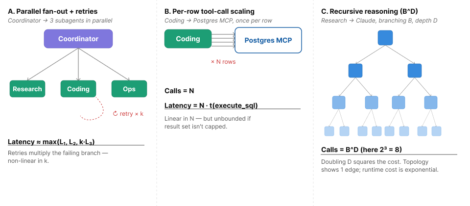
The topology knowledge base captures the relationship that may exist between types of entities, For exaple, a service may be connected to another service, a service may be accessing a database, a service may be layered over a pod.

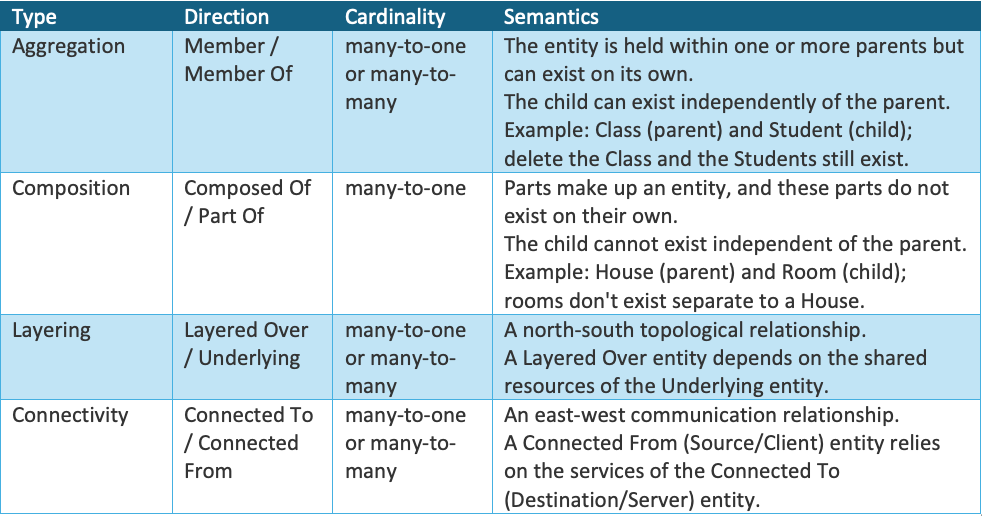
The dynamic topology graph represents the actual discovered relationships between discovered entities. For example, the Coordinator Agent is connected to the Research, Coding, and Ops subagents; the GitHub MCP server, which includes the create pull request tool; and the GPT-4o model, which is layered over the OpenAI model provider (see Figure 1).

It is important to note that the knowledge base captures design-time assertions, not runtime observations. This distinction is critical. A service dependency map derived from trace data reflects what happened during the observation window. The dynamic topology graph reflects what is. Traces may be incomplete (non-instrumented paths, async operations, batch jobs). The dynamic topology graph enables blast-radius analysis; given that entity foo is degraded, which other entities are structurally dependent on it and therefore at risk.

Layer 3: Behavior Model

A behavior model captures the observable signals of normal and abnormal system behavior. It defines symptoms – semantically meaningful deviations from expected state – and events – discrete state transitions that represent changes in entity health or configuration.

A raw metric is not a symptom. The number 95.3 on a CPU utilization gauge is not meaningful without knowing the entity it describes, the threshold at which that utilization constitutes an anomaly, and the operational context in which that threshold applies. A symptom is the semantic interpretation: this entity is exhibiting CPU saturation relative to its configured capacity and expected workload.

The behavior model is what converts monitoring data into an actionable signal. Alerting systems that operate directly on raw metrics without a behavior model produce high false-positive rates because they lack the semantic layer needed to distinguish signal from noise.

The behavior knowledge base captures the possible observable anomalies an entity may experience. For example, a service may be degraded, experiencing high latency, or a node may be highly utilized, experiencing high CPU utilization.

The dynamic behavior model represents the environment's actual runtime state based on what is being observed. For example, the Research subagent is degraded and experiencing high latency, or the Postgres MCP is congested and experiencing high query times.

Layer 4: Causality Model

The causality model captures the cause-and-effect relationship between potential causes and the symptoms or events they may cause.

The causal knowledge base describes the potential causes, the symptoms they may cause, and how they may propagate. Propagation captures how a cause occurring on one entity may propagate to another related entity.  

The causal knowledge base captures generic knowledge about the types of causes that may occur in an environment and how they will manifest, i.e., the symptoms that may be observed when they occur.

For example:

• An MCP service may be congested and when it is congested it may cause its tool calls to be slow, manifested as a high tool-call latency symptom, and may propagate and cause degradation of subagents that depend on it.
• A subagent may be degraded and when it is degraded it may cause its responses to be slow, manifested as a slow response time symptom, and may propagate and cause degradation of the coordinator agent that orchestrates it.
• A model provider may be degraded and when it is degraded it may cause its inference requests to be slow, manifested as high inference latency, and may propagate to subagents using its models causing them to be degraded.

As the above examples illustrate, the causal knowledge base is completely independent of a given environment. It is independent of how many providers, MCP services, and/or subagents are in the environment, and which models run on which providers, which subagents access which MCPs, or which coordinator orchestrates which subagents.

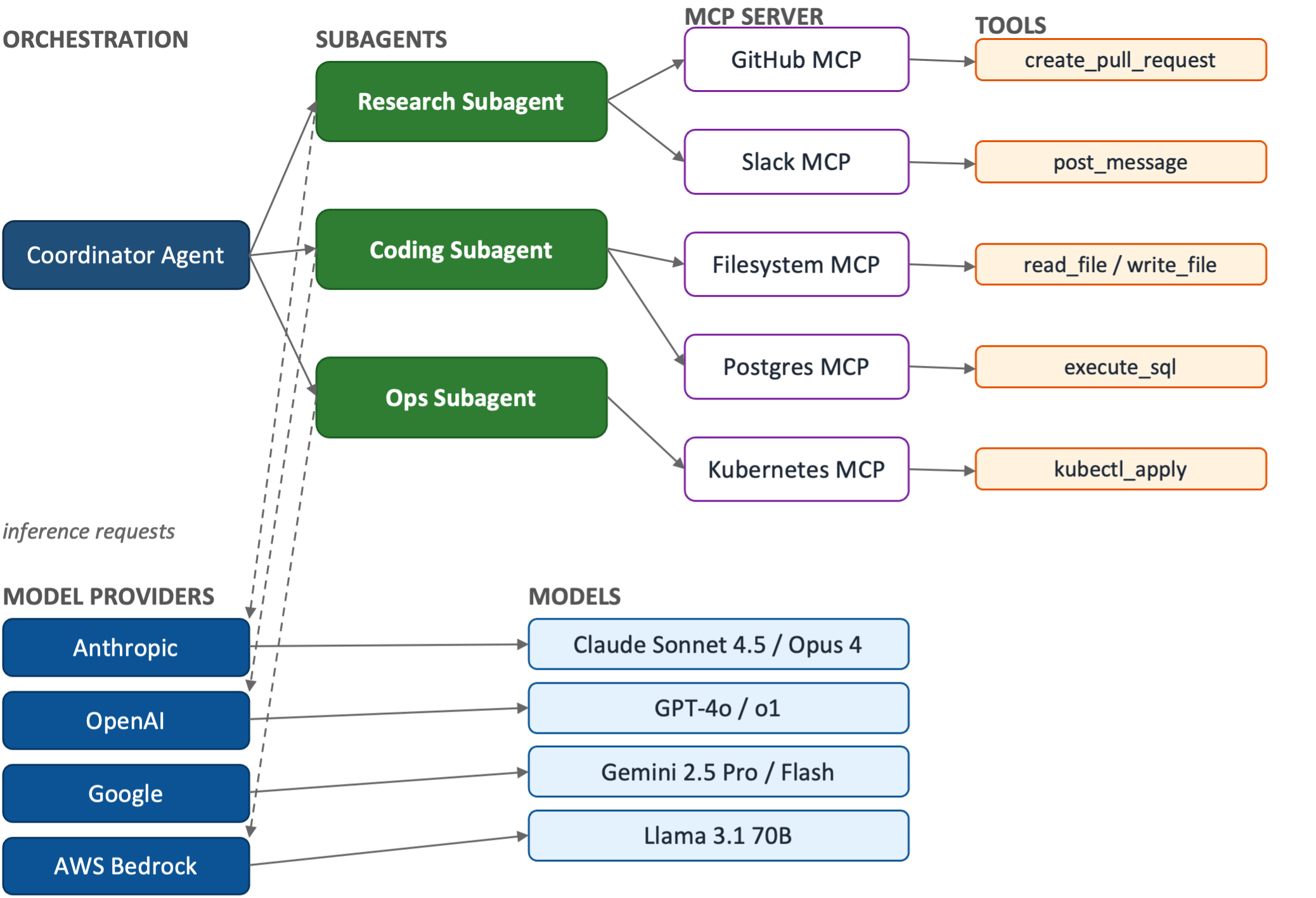
The dynamic causal graph represents the actual runtime causality in the environment at a given point in time. It is a function of the dynamic topology graph and represents all potential specific causes that may occur in the environment, along with the specific symptoms they may cause. The figure below illustrates a concrete example: the Postgres MCP may be congested, and the fault may propagate through the execute_sql tool call to the Coding and Ops subagents, and then onward to the Coordinator, with symptom probability decreasing at each hop. Similarly, Anthropic provider degradation may propagate through Claude inference to the Research, Coding, and Ops subagents, and then to the Coordinator.

In this example, the dynamic causal graph captures that a congested Postgres MCP may cause degradation of the Coding and Ops subagents and the Coordinator. It is important to note that the keyword semantically is “may”. A congested Postgres MCP may degrade downstream entities, but that doesn’t necessarily mean the Postgres MCP is congested – Anthropic provider degradation could produce overlapping symptoms. To conclude, the cause of an observed symptom requires analyzing the state of all potential symptoms.

Cause (left) propagates rightward through topology edges. Probabilities indicate the likelihood of each symptom given the cause. Multiple symptoms may share a cause; diagnosis evaluates the full set of observed symptoms against this graph.

The causality model is what makes root cause analysis tractable. Without it, a single infrastructure fault that produces symptoms across dozens of dependent services generates an alert storm with no structural differentiation between cause and effect. With it, symptoms can be suppressed or annotated as consequences once their cause is pinpointed.

Layer 5: Attributes Dependency Model

Where the causality model operates at the symptom level, the attributes dependency model operates at the attribute level. As its name suggests, it captures attribute dependencies. The dependent attributes can be of the same entity or of different entities. Dependency knowledge captures that attributes are correlated, along with the directionality and function of the correlation. The function can be defined in the model or learned.

The attribute knowledge base captures the generic knowledge of which attribute depends on which. Examples of such dependencies:

• Subagent response latency is a function of the tool-call duration of the MCP services it invokes
• Coordinator response latency is a function of the response latencies of the subagents it orchestrates
• Subagent inference latency is a function of the inference latency of the model provider serving its model
• A subagent's token throughput is a function of the rate at which the coordinator dispatches requests to it.
• The end-to-end coordinator latency is a function of both per-call latencies and the number of subagent calls per task. A non-linear relationship, since a coordinator may fan out to multiple subagents in parallel, retry on failure, or recurse on intermediate results.
• Total tokens consumed by a subagent are a function of both the per-call token cost and the number of model-provider inference calls, which scales non-linearly with conversation depth, tool-call retries, and self-reflection loops.

The dynamic attribute dependency graph represents the actual run-time dependencies in the environment at a given point in time. It is a function of the dynamic topology model. Given the above static model examples, the dynamic model examples would be:

• If the Coding subagent is accessing the Postgres MCP, Coding subagent latency is a function of execute_sql tool-call duration
• If the Coordinator is orchestrating the Coding subagent, Coordinator latency is a function of Coding subagent latency. Note that based on this, Coordinator latency can be computed as a function of execute_sql tool-call duration, even though the Coordinator does not directly access the Postgres MCP.
• If the Research subagent is using Claude served by Anthropic, the Research subagent's inference latency is a function of Anthropic's Claude inference latency.
• For the Ops subagent, its token throughput is a function of the rate of requests the Coordinator dispatches to it.
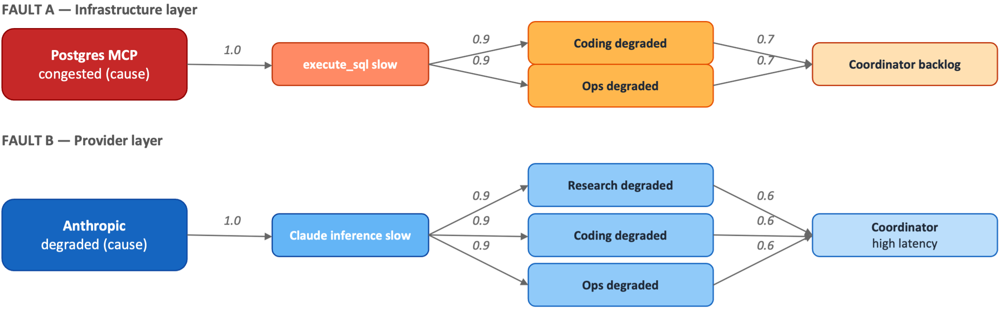
• If the Coordinator fans out a single user task to the Research, Coding, and Ops subagents in parallel, total Coordinator latency is approximately the max of the three subagent latencies, but if any subagent retries on tool-call failure, that subagent's effective latency multiplies by its retry count, so end-to-end latency grows non-linearly with failure rate.
• If the Coding subagent calls the Postgres MCP once per row in a result set, Coding subagent latency is a function of execute_sql duration multiplied by row count, so a query returning N rows produces N tool calls, and end-to-end latency scales with N rather than staying constant.
• If the Research subagent invokes Claude in a multi-turn reasoning loop with branching factor B and depth D, total Anthropic inference calls scale as B^D – so doubling reasoning depth roughly squares the inference cost, even though the Research subagent's per-task topology entry is unchanged.

The attribute dependency graph enables change impact analysis: before modifying a configuration parameter, an operator or automation system can trace the dependency graph to identify which runtime attributes will be affected, on which entities, with what expected magnitude.

Layer 6: Constraint Model

The constraint model defines the desired state. The desired state is one in which goals are achieved while constraints are satisfied. Each entity in an environment may have a desired state, but, more interestingly, the environment as a whole may have one as well.

A desired environment state is one in which all applications deliver on their goals while running within their operational constraints. Usually, the goals are performance goals of latency and throughput, and service level goals in terms of errors and availability, while the operational constraints are capacity, budget, compliance, and configuration.

An entity's desired state is the configuration space within which the entity and its attributes operate without triggering symptoms or degradation events. It is the semantic encoding of the system’s operational envelope.

The constraint model captures both the environment's desired state and the entity's desired state. These can be defined independently, but by using the attribute dependency model, the entity's desired state can be generated/inferred from the environment's desired state, resulting in a very compelling and powerful system.

As in all other layers, the constraint knowledge base captures generic knowledge about constraints, and the dynamic constraint model represents the runtime constraints at a given point in time based on the discovered topology. Constraints are not just thresholds on metrics. They are relationships between configuration parameters and the runtime conditions required for healthy operation:

• Headroom constraint: Container memory limit >= 1.4 x used heap
• Budget constraint: Application cost < budget
• Latency constraint: Service latency < 100ms

When the constraint model is explicit, it becomes possible to answer operational questions that today require senior engineering intuition: “What is the minimum safe memory limit for this service at current traffic?” “If we reduce the connection pool by 40%, at what request rate will we begin to see queuing symptoms?” The constraint model is the missing link between observability (what is happening) and operations (what configuration produces health). It is the semantic layer connecting configuration management to runtime behavior. 

What “Context” Actually Covers and Where It Falls Short

Most observability platforms use the word loosely. Here is what the four common implementations actually encode, and where each one stops.

Shared Labels

Common attributes – service, environment, region, version – are attached to metrics, logs, and traces. This allows tooling to pivot between signal types for a given entity. The relationship is implied by label equality, not by any explicit model of dependency or causation. Two data points sharing service=checkout are navigable together; they are not necessarily related by anything other than that label. This is a partial implementation of the entity model (layer 1) that lacks declarative topological relationships and behavior. 

Topology Map

A topology map encodes structural relationships between entities, which services call which databases, which pods run on which nodes, and which workloads share a cluster. It is the most semantically substantive form of “context” in common tooling and is typically derived from trace data, service-mesh telemetry, or infrastructure APIs. This is a partial implementation of the topology model (layer 2): it captures that entity X is connected to entity Y, but not what behavior propagates along that edge, why a fault on X causes a symptom on Y, or which of X’s attributes drives which of Y’s. A topology map shows the wiring; it does not encode behavior (layer 3), causality (layer 4), attribute dependency (layer 5), or constraints (layer 6). Two services connected in the topology may be tightly coupled in failure propagation or entirely decoupled. The map alone cannot distinguish them. In practice, this means a topology map supports navigation (“show me what this service talks to”) but not reasoning (“if this service degrades, what symptoms should I expect, on which dependents, and why”). That reasoning requires the higher layers.

Temporal Proximity 

Events co-located on a timeline are assumed by operators to be potentially related. The system carries no model of that relationship; pattern recognition is entirely delegated to the human. This is correlation by coincidence, not by structure. It addresses none of the six semantic layers explicitly; it is a UI affordance for human reasoning, not a semantic model.

Distributed Trace Propagation

A trace context header (W3C traceparent, B3, etc.) propagated across service boundaries encodes a genuine causal chain: span B was initiated by span A. This is the most semantically rich form of “context” in common use. It partially implements the topology model (layer 2) for instrumented call paths, and provides raw material for the behavior model (layer 3). However, it is constrained to synchronous, instrumented code paths and does not capture async operations, batch jobs, or infrastructure-level dependencies. It carries no causality, dependency, or constraint models.

In summary, shared labels, temporal proximity, topology, and trace propagation collectively reach into layers 1 and 2. Layers 4 through 6 – causality, dependency, and constraints – are entirely outside the scope of what “context” addresses. That is the gap.

Conclusion 

Context – shared labels, topology map, temporal proximity, trace propagation – is a necessary foundation for navigating observability data. It is not sufficient for understanding systems. The jump from “we can see the signals” to “we understand what is happening and why” requires explicit semantic models at six distinct layers: entity, topology, behavior, causality, dependency, and constraint.

The practical implication for SREs and platform engineers is that runbooks, tribal knowledge, and escalation paths are informal implementations of layers 4 through 6. The question is not whether to encode this knowledge, which already exists, but whether to leave it implicit in human memory or make it explicit in a form that tooling can reason about.

Making semantics explicit is what makes a system legible to an AI agent. An agent reasoning over shared labels, topology, and temporal proximity alone is restricted to the same navigation problem a human faces, pivoting between signals without a model of why they are related. An agent reasoning over layers 4 through 6 can answer the questions that actually drive incident response, capacity planning, and change approval: what is causing this symptom, what is the blast radius of a degraded component, what configuration change would restore the constraint, and what would happen if that change were made. These questions do not require new data; the telemetry, configuration, and trace propagation already carry the raw signal. What they require is a model that the agent can reason against. One that encodes the causal, dependency, and constraint knowledge that today lives only in the engineers who happen to remember.

Semantics is not an observability feature. It is the foundation that makes observability useful.